# load all libraries for this tutorial
#install.packages("datarium")
library(car)
library(datarium)
library(psych)
library(tidyverse)
library(afex)
library(effectsize)
library(emmeans)

Data Preparation

ข้อมูลแบบวัดซ้ำ จัดเป็นข้อมูลเชิงซ้อน (nested data) ประเภทหนึ่ง กล่าวคือ การสังเกตหรือการวัด (observation) แต่ละครั้งซ้อนอยู่ในตัวกลุ่มตัวอย่างแต่ละคน การจัดการข้อมูลเชิงซ้อนนิยมทำในรูปแบบยาว (long format)

ในข้อมูลแบบยาว การสังเกตแต่ละครั้งจะแสดงในแต่ละแถว ข้อมูลจากกลุ่มตัวอย่างคนเดียวกันจะถูกระบุในคอลัมน์ id และการวัดซ้ำแต่ละครั้งจะแสดงด้วยคอลัมน์ Time

ในข้อมูลตัวอย่างนี้ เราใช้ชุดข้อมูล "selfesteem" จาก datarium ซึ่งเป็นข้อมูลคะแนนความภาคภูมิใจในตนเองของกลุ่มตัวอย่างมีจำนวน 10 คน แต่ละคนถูกวัด 3 ครั้ง

หมายเหตุ คำสั่งการวิเคราะห์ใน R เกือบทั้งหมดจะใช้รูปแบบ long format นี้เป็นหลัก ในขณะที่การวิเคราะห์แบบวัดซ้อนในโปรแกรมสถิติอื่น ๆ มักนิยมใช้แบบ wide format (หากสนใจสามารถดูรายละเอียดได้ตอนท้ายของหน้านี้)

Restructure to long format

ข้อมูลแบบกว้างจะวางคะแนนการวัดแต่ละครั้งเป็นคอลัมน์ตัวแปรเรียงต่อกันไป เราจำเป็นต้องแปลงข้อมูลนี้เป็นรูปแบบยาวก่อน

data("selfesteem", package = "datarium")
head(selfesteem) #wide format

## # A tibble: 6 × 4
##      id    t1    t2    t3
##   <int> <dbl> <dbl> <dbl>
## 1     1  4.01  5.18  7.11
## 2     2  2.56  6.91  6.31
## 3     3  3.24  4.44  9.78
## 4     4  3.42  4.71  8.35
## 5     5  2.87  3.91  6.46
## 6     6  2.05  5.34  6.65

ข้อมูลแบบยาว (long format) นี้จะมีตัวแปรอย่างน้อย 3 ตัว ได้แต่ id ของกลุ่มตัวอย่างแต่ละคน Time ครั้งที่วัด และ selfesteem ตัวแปรตามที่ศึกษา

เนื่องจากในกลุ่มตัวอย่าง 10 คน แต่ละคนจะถูกวัด 3 ครั้ง ข้อมูลแบบยาวจะมีทั้งหมด 30 แถว ในรูปแบบ

id	Time	selfesteem
1	Time1	DV_time1
1	Time2	DV_time2
1	Time3	DV_time3
2	Time1	DV_time1
2	Time2	DV_time2
2	Time3	DV_time3
3	…	…
3	…	…
3	…	…
4	…	…
…	…	…

การแปลงข้อมูลแบบกว้างเป็นแบบยาว สามารถทำได้ด้วยคำสั่ง pivot_longer จาก tidyr

se_long <- tidyr::pivot_longer(selfesteem, cols = c("t1", "t2", "t3"), names_to = "Time", values_to = "selfesteem")

se_long$Time <- factor(se_long$Time)
se_long$id <- factor(se_long$id) #VERY IMPORTANT!!! If ID is numerical, the results will be incorrect.
se_long

## # A tibble: 30 × 3
##    id    Time  selfesteem
##    <fct> <fct>      <dbl>
##  1 1     t1          4.01
##  2 1     t2          5.18
##  3 1     t3          7.11
##  4 2     t1          2.56
##  5 2     t2          6.91
##  6 2     t3          6.31
##  7 3     t1          3.24
##  8 3     t2          4.44
##  9 3     t3          9.78
## 10 4     t1          3.42
## # … with 20 more rows
## # ℹ Use `print(n = ...)` to see more rows

Descriptive Statistics

การดูสถิติพื้นฐานทำโดยแบ่งข้อมูลตามตัวแปรวัดซ้ำ Time

describeBy(se_long$selfesteem, group = se_long$Time)

## 
##  Descriptive statistics by group 
## group: t1
##    vars  n mean   sd median trimmed  mad  min  max range  skew kurtosis   se
## X1    1 10 3.14 0.55   3.21    3.17 0.45 2.05 4.01  1.96 -0.45    -0.67 0.17
## ------------------------------------------------------------ 
## group: t2
##    vars  n mean   sd median trimmed mad  min  max range skew kurtosis   se
## X1    1 10 4.93 0.86    4.6    4.81 0.6 3.91 6.91     3 1.01     0.05 0.27
## ------------------------------------------------------------ 
## group: t3
##    vars  n mean   sd median trimmed mad  min  max range skew kurtosis   se
## X1    1 10 7.64 1.14   7.46    7.53 1.4 6.31 9.78  3.47  0.4     -1.3 0.36

Visualization

# Base R
boxplot(selfesteem ~ Time, data = se_long)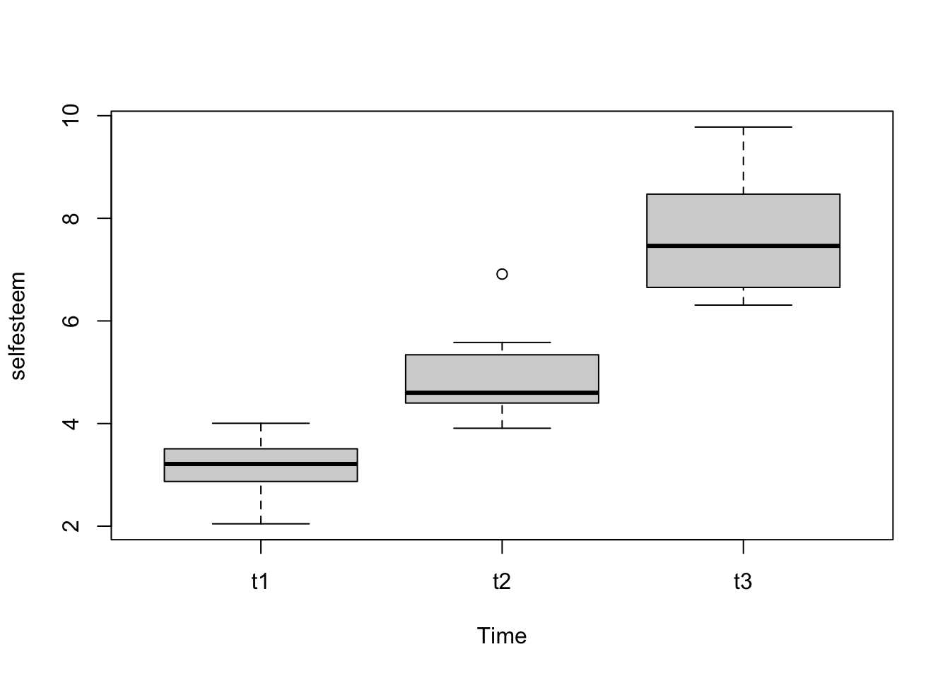

# ggplot2
ggplot(se_long, aes(x = Time, y = selfesteem)) +
  geom_boxplot() +
  theme_classic()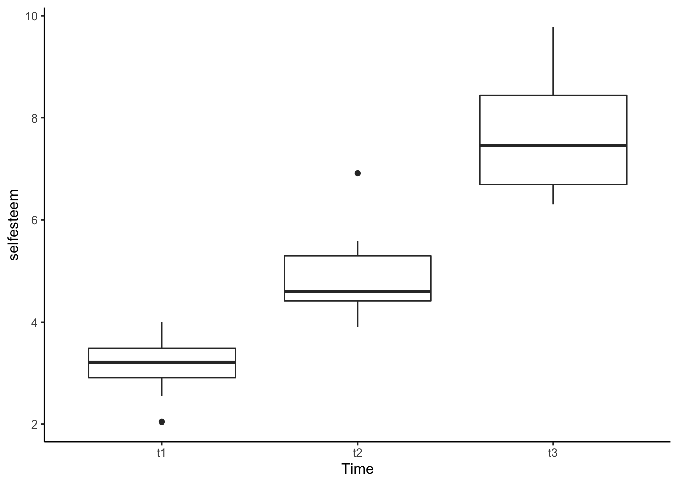

Repeated-Measures ANOVA

`afex` package

การวิเคราะห์ด้วยคำสั่งในแพ็คเกจ afex จะให้รายละเอียดใน output มากกว่า base R

เราสามารถใช้คำสั่ง aov_car() แล้วตามด้วยสูตรโมเดล โดยมีรูปแบบทั่วไปคือ y ~ x + Error(id/x)

x จะเป็นตัวแปรวัดซ้ำ ในตัวอย่างนี้คือ Time
Error() ใช้เพื่อระบุข้อมูลเชิงซ้อน เช่น id/x แสดงว่า ตัวแปร x ซ้อนอยู่ใน id ในที่นี้คือ การวัดแต่ละครั้ง Time ซ้อนอยู่ในกลุ่มตัวอย่างแต่ละคน id แสดงด้วย Error(id/Time)

se.afex <- aov_car(selfesteem ~ Time + Error(id/Time), data = se_long)
summary(se.afex)

## 
## Univariate Type III Repeated-Measures ANOVA Assuming Sphericity
## 
##             Sum Sq num Df Error SS den Df  F value    Pr(>F)    
## (Intercept) 822.72      1   4.5704      9 1620.085 1.795e-11 ***
## Time        102.46      2  16.6237     18   55.469 2.014e-08 ***
## ---
## Signif. codes:  0 '***' 0.001 '**' 0.01 '*' 0.05 '.' 0.1 ' ' 1
## 
## 
## Mauchly Tests for Sphericity
## 
##      Test statistic  p-value
## Time        0.55085 0.092076
## 
## 
## Greenhouse-Geisser and Huynh-Feldt Corrections
##  for Departure from Sphericity
## 
##       GG eps Pr(>F[GG])    
## Time 0.69006  2.161e-06 ***
## ---
## Signif. codes:  0 '***' 0.001 '**' 0.01 '*' 0.05 '.' 0.1 ' ' 1
## 
##         HF eps   Pr(>F[HF])
## Time 0.7743711 6.032582e-07

ค่าสถิติทดสอบให้ดูที่บรรทัด Time ในบรรทัดนี้จะมีทั้งค่า SS_within (Sum Sq) และ SS_error (Error SS)ในบรรทัดเดียวกันเลย

ส่วนค่า SS_between (ความเปลี่ยนแปรที่มาจากความแตกต่างบุคคล) จะอยู่ที่บรรทัด (Intercept) ในส่วนของ Error SS

นอกจากนี้ยังมีการทดสอบ sphericity ให้โดยใช้ Mauchly test รวมไปถึงค่า epsilon ที่ได้จากวิธีประมาณการของ Greenhouse-Geisser และ Huynh-Feldt

หากต้องการค่าสถิติทดสอบที่ปรับแก้แล้วของ Greenhouse-Geisser ให้ใช้คำสั่ง nice() ซึ่งเป็นคำสั่งเฉพาะใน afexคล้ายกับ summary() หากใช้คำสั่งนี้ จะแสดงค่าทดสอบที่ปรับแก้แล้ว (สังเกตว่า df จะถูกปรับให้มีทศนิยม)

nice(se.afex)

## Anova Table (Type 3 tests)
## 
## Response: selfesteem
##   Effect          df  MSE         F  ges p.value
## 1   Time 1.38, 12.42 1.34 55.47 *** .829   <.001
## ---
## Signif. codes:  0 '***' 0.001 '**' 0.01 '*' 0.05 '+' 0.1 ' ' 1
## 
## Sphericity correction method: GG

Normality Assumption with QQ Plot

ใช้คำสั่ง qqPlot() จาก car

qqPlot(residuals(se.afex))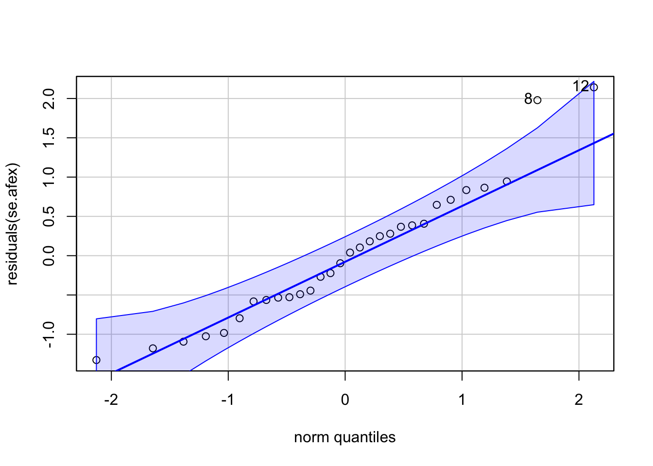

## [1] 12  8

Effect size

eta_squared(se.afex)

## # Effect Size for ANOVA (Type III)
## 
## Parameter | Eta2 (partial) |       95% CI
## -----------------------------------------
## Time      |           0.86 | [0.74, 1.00]
## 
## - One-sided CIs: upper bound fixed at [1.00].

omega_squared(se.afex)

## # Effect Size for ANOVA (Type III)
## 
## Parameter | Omega2 (partial) |       95% CI
## -------------------------------------------
## Time      |             0.81 | [0.64, 1.00]
## 
## - One-sided CIs: upper bound fixed at [1.00].

cohens_f(se.afex)

## # Effect Size for ANOVA (Type III)
## 
## Parameter | Cohen's f (partial) |      95% CI
## ---------------------------------------------
## Time      |                2.48 | [1.67, Inf]
## 
## - One-sided CIs: upper bound fixed at [Inf].

Post-Hoc Analysis

ใช้คำสั่ง emmeans เพื่อสร้าง estimated marginal means ไว้สำหรับทดสอบรายคู่ โดยให้แบ่งการเปรียบเทียบด้วย Time

se.emm <- emmeans(se.afex, ~ Time)
se.emm

##  Time emmean    SE df lower.CL upper.CL
##  t1     3.14 0.174  9     2.75     3.53
##  t2     4.93 0.273  9     4.32     5.55
##  t3     7.64 0.361  9     6.82     8.45
## 
## Confidence level used: 0.95

คำสั่งเปรียบเทียบรายคู่

pairs(se.emm)

##  contrast estimate    SE df t.ratio p.value
##  t1 - t2     -1.79 0.361  9  -4.968  0.0020
##  t1 - t3     -4.50 0.340  9 -13.228  <.0001
##  t2 - t3     -2.70 0.555  9  -4.868  0.0023
## 
## P value adjustment: tukey method for comparing a family of 3 estimates

Contrast

การทดสอบ contrast เฉพาะรายคู่ที่กำหนด ให้สร้าง contrast matrix contrast_m ขึ้นมาเพื่อกำหนดคู่ที่ต้องการจะเทียบ

หมายเหตุ การเรียงลำดับน้ำหนัก ต้องเรียงตาม level ของ factor ดูคำสั่ง str()

contrast_m <- data.frame("t1 vs t23"  = c(-1,  1/2, 1/2),
                         "t1 vs t3"   = c( 1,    0,  -1),
                         row.names = c("t1", "t2", "t3"))
contrast_m

##    t1.vs.t23 t1.vs.t3
## t1      -1.0        1
## t2       0.5        0
## t3       0.5       -1

contrast(se.emm, method = contrast_m, adjust = "sidak", infer = TRUE)

##  contrast  estimate    SE df lower.CL upper.CL t.ratio p.value
##  t1.vs.t23     3.15 0.214  9     2.57     3.72  14.678  <.0001
##  t1.vs.t3     -4.50 0.340  9    -5.41    -3.59 -13.228  <.0001
## 
## Confidence level used: 0.95 
## Conf-level adjustment: sidak method for 2 estimates 
## P value adjustment: sidak method for 2 tests

Extra

Long Format with Base R `aov()`

โมเดล aov สำหรับข้อมูลวัดซ้ำจะมีรูปแบบทั่วไปคือ y ~ x + Error(id/x)

x จะเป็นตัวแปรวัดซ้ำ ในตัวอย่างนี้คือ Time

Error() ใช้เพื่อระบุข้อมูลเชิงซ้อน เช่น id/x แสดงว่า ตัวแปร x ซ้อนอยู่ใน id ในที่นี้คือ การวัดแต่ละครั้ง Time ซ้อนอยู่ในกลุ่มตัวอย่างแต่ละคน id แสดงด้วย Error(id/Time)

se.aov <- aov(selfesteem ~ Time + Error(id/Time), data = se_long)
summary(se.aov)

## 
## Error: id
##           Df Sum Sq Mean Sq F value Pr(>F)
## Residuals  9   4.57  0.5078               
## 
## Error: id:Time
##           Df Sum Sq Mean Sq F value   Pr(>F)    
## Time       2 102.46   51.23   55.47 2.01e-08 ***
## Residuals 18  16.62    0.92                     
## ---
## Signif. codes:  0 '***' 0.001 '**' 0.01 '*' 0.05 '.' 0.1 ' ' 1

อย่างไรก็ดีคำสั่ง aov_car จาก afex ให้ผล summary ที่ละเอียดกว่า จึงแนะนำให้ใช้ afex แทน

Wide Format

library(jmv)

ข้อมูลแบบวัดซ้ำ (repeated measures) สามารถจัดได้สองแบบ คือ แบบกว้าง (wide format) และแบบยาว (long format)

ในการจัดข้อมูลแบบกว้าง แต่ละแถว (row) จะแทนกลุ่มตัวอย่างแต่ละคน ข้อมูลตัวแปรตามที่วัดซ้ำจะแทนด้วยคอลัมน์ตามจำนวนการวัด ดังตัวอย่างด้านล่าง

data("selfesteem", package = "datarium")
head(selfesteem)

## # A tibble: 6 × 4
##      id    t1    t2    t3
##   <int> <dbl> <dbl> <dbl>
## 1     1  4.01  5.18  7.11
## 2     2  2.56  6.91  6.31
## 3     3  3.24  4.44  9.78
## 4     4  3.42  4.71  8.35
## 5     5  2.87  3.91  6.46
## 6     6  2.05  5.34  6.65

ข้อมูลแบบกว้างเป็นการจัดข้อมูลที่นิยมใช้ใน repeated ANOVA ของโปรแกรมสถิติทั่วไป เช่น SPSS, jamovi

Descriptive Statistics

การเรียกดูค่าสถิติพื้นฐานในข้อมูลแบบกว้างนี้สามารถทำเหมือนกับการเรียกดูข้อมูลของตัวแปร (คอลัมน์) แต่ละตัว

psych::describe(selfesteem[,c("t1", "t2", "t3")])

##    vars  n mean   sd median trimmed  mad  min  max range  skew kurtosis   se
## t1    1 10 3.14 0.55   3.21    3.17 0.45 2.05 4.01  1.96 -0.45    -0.67 0.17
## t2    2 10 4.93 0.86   4.60    4.81 0.60 3.91 6.91  3.00  1.01     0.05 0.27
## t3    3 10 7.64 1.14   7.46    7.53 1.40 6.31 9.78  3.47  0.40    -1.30 0.36

Boxplot

boxplot(selfesteem[,c("t1", "t2", "t3")])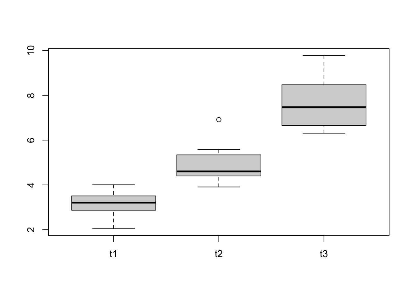

Normality Assumption

shapiro.test(selfesteem$t1)

## 
##  Shapiro-Wilk normality test
## 
## data:  selfesteem$t1
## W = 0.96669, p-value = 0.8586

shapiro.test(selfesteem$t2)

## 
##  Shapiro-Wilk normality test
## 
## data:  selfesteem$t2
## W = 0.87588, p-value = 0.117

shapiro.test(selfesteem$t3)

## 
##  Shapiro-Wilk normality test
## 
## data:  selfesteem$t3
## W = 0.92271, p-value = 0.3802

สำหรับ QQ plot เราจะใช้คำสั่ง qqPlot (P ตัวใหญ่) จาก package car

car::qqPlot(selfesteem$t1)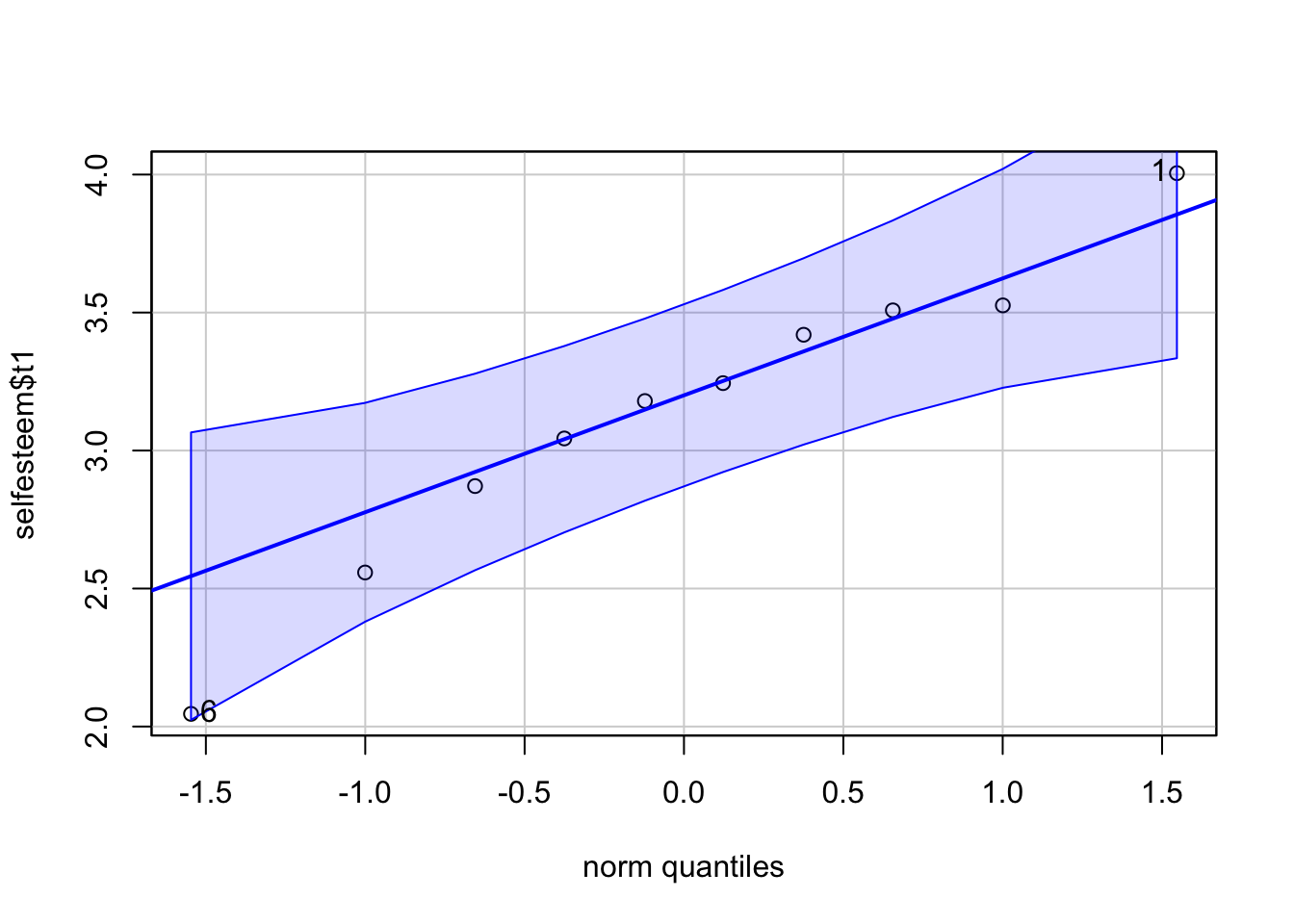

## [1] 6 1

qqPlot(selfesteem$t2)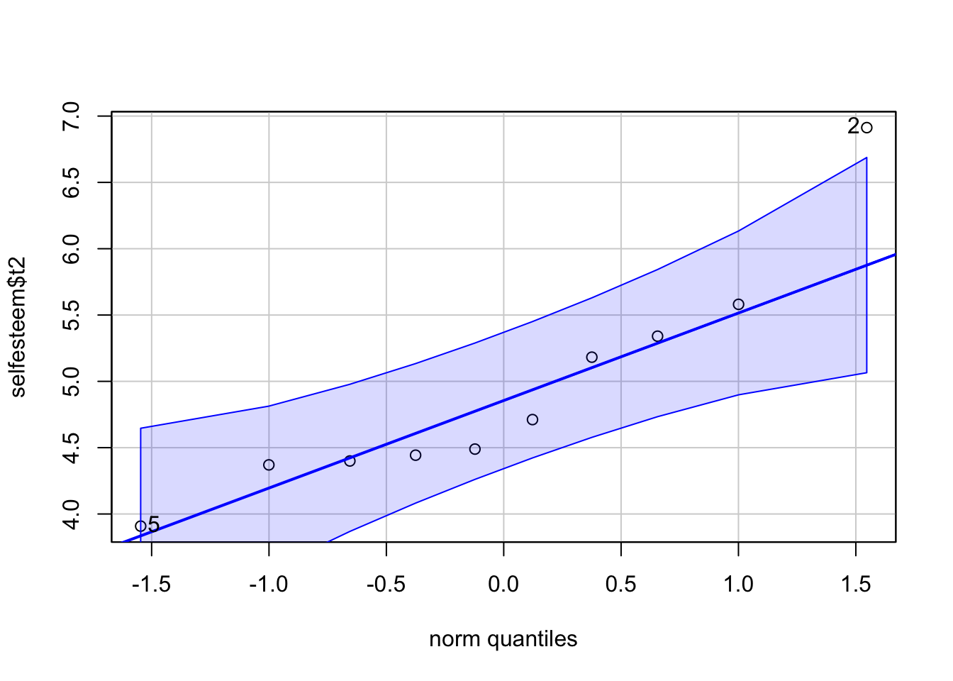

## [1] 2 5

qqPlot(selfesteem$t3)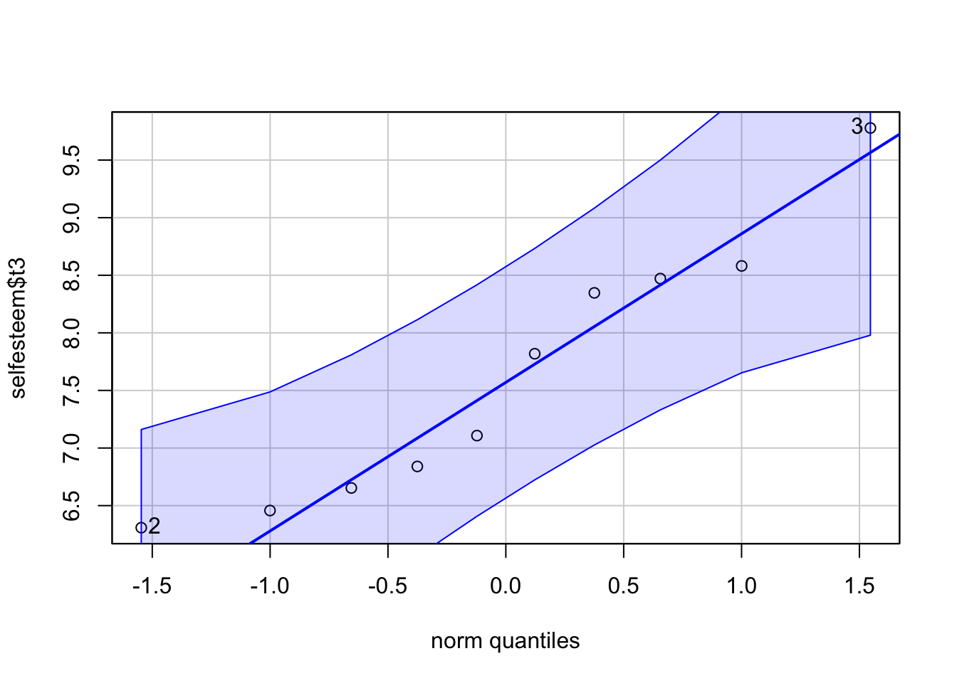

## [1] 3 2

`jmv` Package

การวิเคราะห์ข้อมูลวัดซ้ำใน R นั้นมักจะวิเคราะห์ด้วย long format จึงไม่มีคำสั่ง Base R สำหรับวิเคราะห์ข้อมูลแบบ wide format

ถ้าต้องการวิเคราะห์ด้วย wide format เราสามารถใช้คำสั่ง anovaRM ใน package jmv ได้

โดยต้องกำหนด option หลัก 3 ตัว คือ rm, rmCells, และ rmTerms

ใน rm จะกำหนด label = ชื่อตัวแปรวัดซ้ำ เช่น เวลา/เงื่อนไข/ขนาดโดสยา/อื่นๆ และ levels = ชื่อระดับตัวแปรวัดซ้ำ

ใน rmCells จะกำหนด measure = ชื่อตัวแปรในข้อมูล คู่กับ cell = ชื่อ level ที่ตรงกัน

ส่วน rmTerms คือการกำหนดว่า effect ตัวไหนจะเป็นอิทธิพลแบบภายในบุคคล (within-subject)

jmv::anovaRM(data = selfesteem, 
            rm = list(
                      list(
                          label = "Time",
                          levels = c("Time 1","Time 2","Time 3")
                          )),
             rmCells=list(
                       list(
                           measure="t1",
                           cell = "Time 1"),
                       list(
                           measure="t2",
                           cell = "Time 2"),
                      list(
                           measure="t3",
                           cell = "Time 3")),
             rmTerms = ~ Time,
             effectSize = "partEta",
             spherTest = TRUE)

## 
##  REPEATED MEASURES ANOVA
## 
##  Within Subjects Effects                                                                    
##  ────────────────────────────────────────────────────────────────────────────────────────── 
##                Sum of Squares    df    Mean Square    F           p             η²-p        
##  ────────────────────────────────────────────────────────────────────────────────────────── 
##    Time             102.45582     2     51.2279125    55.46903    < .0000001    0.8603981   
##    Residual          16.62374    18      0.9235409                                          
##  ────────────────────────────────────────────────────────────────────────────────────────── 
##    Note. Type 3 Sums of Squares
## 
## 
##  Between Subjects Effects                                                           
##  ────────────────────────────────────────────────────────────────────────────────── 
##                Sum of Squares    df    Mean Square    F    p            η²-p        
##  ────────────────────────────────────────────────────────────────────────────────── 
##    Residual          4.570442     9      0.5078269                                  
##  ────────────────────────────────────────────────────────────────────────────────── 
##    Note. Type 3 Sums of Squares
## 
## 
##  ASSUMPTIONS
## 
##  Tests of Sphericity                                                           
##  ───────────────────────────────────────────────────────────────────────────── 
##            Mauchly's W    p            Greenhouse-Geisser ε    Huynh-Feldt ε   
##  ───────────────────────────────────────────────────────────────────────────── 
##    Time      0.5508534    0.0920755               0.6900613        0.7743711   
##  ─────────────────────────────────────────────────────────────────────────────

หากต้องการค่าสถิติของ Greenhouse-Geisser ที่มีการปรับแก้ค่า df

jmv::anovaRM(data = selfesteem, 
            rm = list(
                      list(
                          label = "Time",
                          levels = c("Time 1","Time 2","Time 3")
                          )),
             rmCells=list(
                       list(
                           measure="t1",
                           cell = "Time 1"),
                       list(
                           measure="t2",
                           cell = "Time 2"),
                      list(
                           measure="t3",
                           cell = "Time 3")),
             rmTerms = ~ Time,
             spherTest = TRUE,
             spherCorr = "GG")

## 
##  REPEATED MEASURES ANOVA
## 
##  Within Subjects Effects                                                                                      
##  ──────────────────────────────────────────────────────────────────────────────────────────────────────────── 
##                Sphericity Correction    Sum of Squares    df           Mean Square    F           p           
##  ──────────────────────────────────────────────────────────────────────────────────────────────────────────── 
##    Time        Greenhouse-Geisser            102.45582     1.380123      74.236755    55.46903    0.0000022   
##    Residual    Greenhouse-Geisser             16.62374    12.421104       1.338346                            
##  ──────────────────────────────────────────────────────────────────────────────────────────────────────────── 
##    Note. Type 3 Sums of Squares
## 
## 
##  Between Subjects Effects                                              
##  ───────────────────────────────────────────────────────────────────── 
##                Sum of Squares    df    Mean Square    F    p           
##  ───────────────────────────────────────────────────────────────────── 
##    Residual          4.570442     9      0.5078269                     
##  ───────────────────────────────────────────────────────────────────── 
##    Note. Type 3 Sums of Squares
## 
## 
##  ASSUMPTIONS
## 
##  Tests of Sphericity                                                           
##  ───────────────────────────────────────────────────────────────────────────── 
##            Mauchly's W    p            Greenhouse-Geisser ε    Huynh-Feldt ε   
##  ───────────────────────────────────────────────────────────────────────────── 
##    Time      0.5508534    0.0920755               0.6900613        0.7743711   
##  ─────────────────────────────────────────────────────────────────────────────

Lab 10: Repeated-Measures ANOVA

Data Preparation

Restructure to long format

Descriptive Statistics

Visualization

Repeated-Measures ANOVA

afex package

Normality Assumption with QQ Plot

Effect size

Post-Hoc Analysis

Contrast

Extra

Long Format with Base R aov()

Wide Format

Descriptive Statistics

Boxplot

Normality Assumption

jmv Package

`afex` package

Long Format with Base R `aov()`

`jmv` Package