Lab 13: Analysis of Covariance
# load all libraries for this tutorial
library(datarium)
library(dplyr)
library(emmeans)
library(afex)
library(ggplot2)
Tutorial นี้จะแสดงวิธีการวิเคราะห์ความแปรปรวนร่วม (ANCOVA)
One-Way ANCOVA
ในตัวอย่างนี้ เราจะใช้ข้อมูล stress จาก datarium package
ข้อมูลนี้เป็นการทดลองว่า treatment และ exercise
มีผลต่อ score หรือไม่ โดยมี age เป็นตัวแปรร่วม
(covariate)
ตัวแปรทุกตัวได้รับตั้งค่าประเภทตัวแปรแล้ว
data(stress)
str(stress)
## tibble [60 × 5] (S3: tbl_df/tbl/data.frame)
## $ id : int [1:60] 1 2 3 4 5 6 7 8 9 10 ...
## $ score : num [1:60] 95.6 82.2 97.2 96.4 81.4 83.6 89.4 83.8 83.3 85.7 ...
## ..- attr(*, "label")= chr "Cholesterol concentration (in mmol/L)"
## ..- attr(*, "format.spss")= chr "F8.2"
## ..- attr(*, "display_width")= int 9
## $ treatment: Factor w/ 2 levels "yes","no": 1 1 1 1 1 1 1 1 1 1 ...
## $ exercise : Factor w/ 3 levels "low","moderate",..: 1 1 1 1 1 1 1 1 1 1 ...
## $ age : num [1:60] 59 65 70 66 61 65 57 61 58 55 ...
## ..- attr(*, "label")= chr "Body weight (in kg)"
## ..- attr(*, "format.spss")= chr "F8.2"Model
เราจะใช้ทำสั่ง aov_car จาก afex package
ในการวิเคราะห์ความแปรปรวนร่วมทางเดียว
เราจะใช้ treatment เป็นตัวแปรอิสระ และ age เป็น
covariate (ยังไม่ต้องสนตัวแปร exercise)
โมเดล คือ ตัวแปรสองตัวนี้ร่วมกันอธิบายตัวแปรตาม score จึงใช้
treatment + age
ใช้ option factorize = FALSE เนื่องจากคำสั่ง
aov_car จะแปลงตัวแปรทุกตัวในโมเดลเป็น factor โดยอัตโนมัติ
เผื่อในกรณีที่ผู้ใช้ลืมแปลงตัวแปรเป็น factor (ถ้าหากไม่กำหนด
factorize = FALSE คำสั่ง aov_car จะพยายามแปลง
age เป็น factor แล้วทำให้เกิด error)
one.ancova.afex <- aov_car(score ~ treatment + age + Error(id), data = stress, factorize = FALSE)## Warning: Numerical variables NOT centered on 0 (i.e., likely bogus results): age## Contrasts set to contr.sum for the following variables: treatmentsummary(one.ancova.afex)## Anova Table (Type 3 tests)
##
## Response: score
## num Df den Df MSE F ges Pr(>F)
## treatment 1 57 45.132 4.9182 0.079431 0.03058 *
## age 1 57 45.132 21.3676 0.272658 2.218e-05 ***
## ---
## Signif. codes: 0 '***' 0.001 '**' 0.01 '*' 0.05 '.' 0.1 ' ' 1nice(one.ancova.afex, es = "pes") #short summary with partial eta square## Anova Table (Type 3 tests)
##
## Response: score
## Effect df MSE F pes p.value
## 1 treatment 1, 57 45.13 4.92 * .079 .031
## 2 age 1, 57 45.13 21.37 *** .273 <.001
## ---
## Signif. codes: 0 '***' 0.001 '**' 0.01 '*' 0.05 '+' 0.1 ' ' 1จะเห็นว่ามีคำเตือนว่าตัวแปรเชิงตัวเลข ไม่ถูกแปลงเป็นค่ากึ่งกลาง (centered variable;
ค่าตัวแปรที่ลบออกด้วยค่าเฉลี่ยของตัวมันเอง) การแปลงเป็นค่ากึ่งกลางจะช่วยให้ค่า intercept
แสดงถึงค่าเฉลี่ยของกลุ่มอ้างอิง (reference group) เมื่อควบคุมให้ covariate อยู่ที่ค่าเฉลี่ย
ซึ่งไม่ใช่สิ่งที่เราสนใจในกรณีนี้ เราจึงไม่ต้องสนใจคำเตือนนี้ก็ได้
(หากต้องการลองวิเคราะห์โดยใช้ค่าที่ center แล้ว สามารถใช้คำสั่ง
scale(x, center = TRUE, scale = FALSE) เพื่อแปลงตัวแปร
age เป็นค่ากึ่งกลางก่อนนำไปวิเคราะห์ข้อมูล)
# In one-way ANCOVA, centered covariate produce the same result as uncentered covariate.
stress$cen.age <- scale(stress$age, scale = FALSE)
center.afex <- aov_car(score ~ treatment + cen.age + Error(id), data = stress, factorize = FALSE)
## Contrasts set to contr.sum for the following variables: treatmentsummary(center.afex)## Anova Table (Type 3 tests)
##
## Response: score
## num Df den Df MSE F ges Pr(>F)
## treatment 1 57 45.132 4.9182 0.079431 0.03058 *
## cen.age 1 57 45.132 21.3676 0.272658 2.218e-05 ***
## ---
## Signif. codes: 0 '***' 0.001 '**' 0.01 '*' 0.05 '.' 0.1 ' ' 1nice(center.afex, es = "pes") #short summary with partial eta square## Anova Table (Type 3 tests)
##
## Response: score
## Effect df MSE F pes p.value
## 1 treatment 1, 57 45.13 4.92 * .079 .031
## 2 cen.age 1, 57 45.13 21.37 *** .273 <.001
## ---
## Signif. codes: 0 '***' 0.001 '**' 0.01 '*' 0.05 '+' 0.1 ' ' 1Pairwise Comparisons
ค่าเฉลี่ยประมาณตามขอบ (estimated marginal means)
เป็นค่าเฉลี่ยของเงื่อนไขแต่ละกลุ่มเมื่อควบคุมค่าตัวแปรร่วม age
ให้คงที่ที่ค่าเฉลี่ยของตัวมันเอง นั่นคือ หากทั้งสองเงื่อนไขมีอายุเท่ากันที่ 59.95 ปี
ค่าเฉลี่ยของตัวแปรตาม score ของแต่ละกลุ่มจะเป็นเท่าใด
สังเกตว่าค่า emmeans และค่าเฉลี่ยที่ยังไม่ปรับของแต่ละกลุ่ม จะแตกต่างกันเล็กน้อย
by(stress$score, stress$treatment, mean) # raw (unadjusted mean)## stress$treatment: yes
## [1] 82.15667
## ------------------------------------------------------------
## stress$treatment: no
## [1] 86.99667one.ancova.emm <- emmeans(one.ancova.afex, ~ treatment)
summary(one.ancova.emm) # estimated (adjusted) mean## treatment emmean SE df lower.CL upper.CL
## yes 82.6 1.23 57 80.2 85.1
## no 86.5 1.23 57 84.0 89.0
##
## Confidence level used: 0.95pairs(one.ancova.emm) #pairwise comparison of adjusted means## contrast estimate SE df t.ratio p.value
## yes - no -3.87 1.75 57 -2.218 0.0306Plot
emm.summary <- summary(one.ancova.emm)
ggplot(emm.summary, aes(x = treatment, y = emmean)) +
  geom_point() +
  geom_line(aes(group = 1), linetype = "dashed") + #group = 1 for having only one factor (treatment) in the plot
  geom_errorbar(aes(ymin = lower.CL, ymax = upper.CL), width = .3) +
  xlab("Treatment") +
  ylab("Score") +
  ylim(c(50,100)) + #start Y-axid at score = 50
  theme_classic()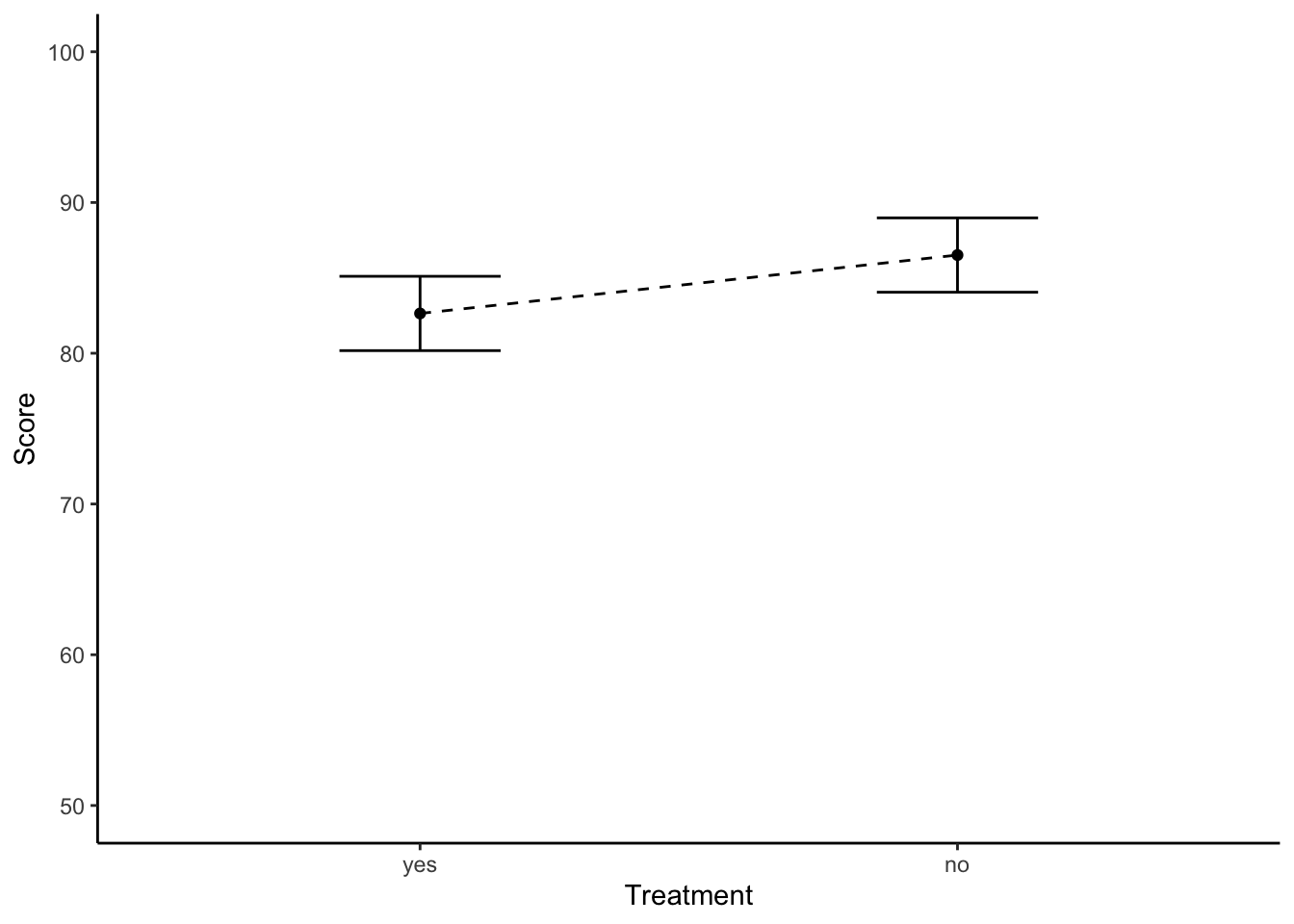
Homogeneity of Regression Assumptions
การวิเคราะห์ความแปรปรวนร่วม มีข้อสมมติพื้นฐานข้อหนึ่งคือ ค่า slope ระหว่างตัวแปรร่วมและตัวแปรตาม จะเท่ากันในทุกเงื่อนไขของตัวแปรอิสระ กล่าวคือ slope ของ covariate และ DV ในแต่ละเงื่อนไขการทดลองจะต้องขนานกัน
การที่ slope ขนานกันในทุกเงื่อนไขคือการบอกว่าตัวแปรอิสระและตัวแปรร่วม นั้นไม่มีปฏิสัมพันธ์กัน
เราสามารถทดสอบได้โดยการสร้างโมเดลที่มีการทดสอบปฏิสัมพันธ์ของตัวแปรอิสระและตัวแปรร่วม
treatment * age
one.ancova.afex2 <- aov_car(score ~ treatment * age + Error(id), data = stress, factorize = FALSE)## Warning: Numerical variables NOT centered on 0 (i.e., likely bogus results): age## Contrasts set to contr.sum for the following variables: treatmentsummary(one.ancova.afex2)## Anova Table (Type 3 tests)
##
## Response: score
## num Df den Df MSE F ges Pr(>F)
## treatment 1 56 44.453 2.3110 0.039633 0.1341
## age 1 56 44.453 23.5415 0.295965 1.015e-05 ***
## treatment:age 1 56 44.453 1.8705 0.032322 0.1769
## ---
## Signif. codes: 0 '***' 0.001 '**' 0.01 '*' 0.05 '.' 0.1 ' ' 1เราพบว่าปฏิสัมพันธ์ระหว่างตัวแปรอิสระและตัวแปรร่วมไม่มีนัยสำคัญทางสถิติ
ข้อสมมติฐานพื้นฐานนี้ไม่ถูกละเมิด เราจึงเลือกที่จะใช้ผลจากการวิเคราะห์ ANCOVA
one.ancova.afex ตัวแรกด้านบน
Two-way ANCOVA
Model
การวิเคราะห์ตัวแปรร่วมสามารถทำใน factorial design ก็ได้ ใน factorial design
นี้มีตัวแปรอิสระแบบจัดประเภทสองตัว คือ treatment และ
exercise ส่วนตัวแปรร่วมคือ age
two.ancova <- aov_car(score ~ treatment * exercise + age + Error(id), data = stress, factorize = FALSE)## Warning: Numerical variables NOT centered on 0 (i.e., likely bogus results): age## Contrasts set to contr.sum for the following variables: treatment, exercisesummary(two.ancova)## Anova Table (Type 3 tests)
##
## Response: score
## num Df den Df MSE F ges Pr(>F)
## treatment 1 53 24.848 11.0657 0.17272 0.001603 **
## exercise 2 53 24.848 20.7147 0.43873 2.254e-07 ***
## age 1 53 24.848 9.1097 0.14667 0.003903 **
## treatment:exercise 2 53 24.848 4.4458 0.14366 0.016409 *
## ---
## Signif. codes: 0 '***' 0.001 '**' 0.01 '*' 0.05 '.' 0.1 ' ' 1nice(two.ancova, es = "pes")## Anova Table (Type 3 tests)
##
## Response: score
## Effect df MSE F pes p.value
## 1 treatment 1, 53 24.85 11.07 ** .173 .002
## 2 exercise 2, 53 24.85 20.71 *** .439 <.001
## 3 age 1, 53 24.85 9.11 ** .147 .004
## 4 treatment:exercise 2, 53 24.85 4.45 * .144 .016
## ---
## Signif. codes: 0 '***' 0.001 '**' 0.01 '*' 0.05 '+' 0.1 ' ' 1Homogeneity of regression
two.ancova2 <- aov_car(score ~ treatment * exercise * age + Error(id), data = stress, factorize = FALSE)## Warning: Numerical variables NOT centered on 0 (i.e., likely bogus results): age## Contrasts set to contr.sum for the following variables: treatment, exercisesummary(two.ancova2)## Anova Table (Type 3 tests)
##
## Response: score
## num Df den Df MSE F ges Pr(>F)
## treatment 1 48 27.08 0.0650 0.001351 0.79991
## exercise 2 48 27.08 0.0900 0.003734 0.91413
## age 1 48 27.08 4.5622 0.086796 0.03781 *
## treatment:exercise 2 48 27.08 0.1097 0.004549 0.89634
## treatment:age 1 48 27.08 0.0082 0.000171 0.92821
## exercise:age 2 48 27.08 0.0745 0.003094 0.92834
## treatment:exercise:age 2 48 27.08 0.0730 0.003034 0.92967
## ---
## Signif. codes: 0 '***' 0.001 '**' 0.01 '*' 0.05 '.' 0.1 ' ' 1ตัวแปร age ไม่มีปฏิสัมพันธ์กับตัวแปรอิสระใด ๆ และไม่มีปฏิสัมพันธ์สามทาง จึงไม่ละเมิดเรื่อง
homogeneity of regression เราจึงเลือกใช้ผลการวิเคราะห์จาก โมเดล ANCOVA
treatment * exercise + age ได้
Simple Effects
ค่าเฉลี่ยประมาณตามขอบในการวิเคราะห์นี้เป็นค่าตัวแปรตามที่ถูกควบคุมเมื่อตัวแปรร่วม
age คงที่อยู่ที่ค่าเฉลี่ย
วิธีการสร้าง emmeans และการเปรียบเทียบรายคู่ ทำเหมือน factorial ANOVA ตามปกติ ค่าที่ได้จะเป็นค่าจากโมเดลซึ่งควบคุมตัวแปรร่วมแล้ว
two.ancova.emm <- emmeans(two.ancova, ~ treatment | exercise)
summary(two.ancova.emm) #adjusted (estimated) marginal means
## exercise = low:
## treatment emmean SE df lower.CL upper.CL
## yes 87.0 1.60 53 83.8 90.2
## no 88.5 1.62 53 85.3 91.7
##
## exercise = moderate:
## treatment emmean SE df lower.CL upper.CL
## yes 87.0 1.58 53 83.8 90.2
## no 88.7 1.59 53 85.5 91.9
##
## exercise = high:
## treatment emmean SE df lower.CL upper.CL
## yes 73.3 1.65 53 70.0 76.6
## no 83.0 1.61 53 79.8 86.3
##
## Confidence level used: 0.95pairs(two.ancova.emm, simple = "treatment") #simple effect of treatment by exercise groups## exercise = low:
## contrast estimate SE df t.ratio p.value
## yes - no -1.53 2.23 53 -0.685 0.4961
##
## exercise = moderate:
## contrast estimate SE df t.ratio p.value
## yes - no -1.68 2.25 53 -0.748 0.4575
##
## exercise = high:
## contrast estimate SE df t.ratio p.value
## yes - no -9.75 2.23 53 -4.362 0.0001pairs(two.ancova.emm, simple = "exercise") #simple effect of treatment by exercise groups## treatment = yes:
## contrast estimate SE df t.ratio p.value
## low - moderate -0.0175 2.26 53 -0.008 1.0000
## low - high 13.7033 2.36 53 5.799 <.0001
## moderate - high 13.7208 2.27 53 6.042 <.0001
##
## treatment = no:
## contrast estimate SE df t.ratio p.value
## low - moderate -0.1725 2.23 53 -0.077 0.9967
## low - high 5.4851 2.34 53 2.347 0.0579
## moderate - high 5.6576 2.30 53 2.455 0.0451
##
## P value adjustment: tukey method for comparing a family of 3 estimatesCustomize Covariate Value
หากต้องการประมาณค่าเฉลี่ยตามขอบ (ค่าเฉลี่ยของแต่ละเงื่อนไข)
โดยกำหนดค่าตัวแปรควบคุมเป็นค่าอื่น สามารถใช้ option at = list()
กำหนดค่าของตัวแปรควบคุมที่ต้องการได้
at30.emm <- emmeans(two.ancova, ~ treatment | exercise, at = list(age = 30))
at30.emm #notice slight changes in emmeans
## exercise = low:
## treatment emmean SE df lower.CL upper.CL
## yes 71.9 5.52 53 60.8 83.0
## no 73.4 5.58 53 62.2 84.6
##
## exercise = moderate:
## treatment emmean SE df lower.CL upper.CL
## yes 71.9 5.18 53 61.5 82.3
## no 73.6 5.47 53 62.6 84.6
##
## exercise = high:
## treatment emmean SE df lower.CL upper.CL
## yes 58.2 4.77 53 48.6 67.8
## no 67.9 4.91 53 58.1 77.8
##
## Confidence level used: 0.95pairs(at30.emm, simple = "treatment") #but the model is linear. All estimated means differences will be the same at any value of covariate. ## exercise = low:
## contrast estimate SE df t.ratio p.value
## yes - no -1.53 2.23 53 -0.685 0.4961
##
## exercise = moderate:
## contrast estimate SE df t.ratio p.value
## yes - no -1.68 2.25 53 -0.748 0.4575
##
## exercise = high:
## contrast estimate SE df t.ratio p.value
## yes - no -9.75 2.23 53 -4.362 0.0001สังเกตว่าค่า emmean ของแต่ละกลุ่มเปลี่ยนไปจากด้านบน
เนื่องจากเรากำหนดให้ค่า covariate เป็น 30 ปี (แทนที่จะเป็นค่าเฉลี่ย 59.95 ปี)
อย่างไรก็ดีการทดสอบ simple effect จะได้ผลเท่าเดิม เนื่องจากในโมเดลนี้ covariate
ถูกกำหนดให้สัมพันธ์เชิงเส้นตรงกับตัวแปรตามและไม่มีปฏิสัมพันธ์กับตัวแปรอิสระ
ดังนั้นอิทธิพลของตัวแปรอิสระจะมีค่าคงเดิมในทุก ๆ ค่าของตัวเแปร covariate
(ไม่ว่าอายุจะเป็นเท่าไหร่ อิทธิพลของ treatment และ
exercise ต่อ score ก็ยังเท่าเดิมเสมอในทุกช่วงอายุ)
Copyright © 2022 Kris Ariyabuddhiphongs